Código
%%capture
# DARTS now is lightweight install: please see
# https://github.com/unit8co/darts/blob/master/INSTALL.md#enabling-optional-dependencies
# Descomente se for rodar pela primeira vez:
!pip install darts prophet statsforecastReferências: - https://unit8.com/resources/darts-time-series-made-easy-in-python/ - https://levelup.gitconnected.com/a-python-library-that-makes-it-simple-to-forecast-time-series-6a403da71542 - https://pypi.org/project/statsforecast/
%%capture
# DARTS now is lightweight install: please see
# https://github.com/unit8co/darts/blob/master/INSTALL.md#enabling-optional-dependencies
# Descomente se for rodar pela primeira vez:
!pip install darts prophet statsforecastfrom darts.models import (
NaiveSeasonal,
NaiveDrift,
Prophet,
ExponentialSmoothing,
ARIMA,
AutoARIMA,
TBATS
)
from darts import TimeSeries
from darts.metrics import mape, mase, mae, mse, ope, r2_score, rmse, rmsle
from statsmodels.tsa.stattools import adfuller
import time
import pandas as pd
import numpy as np
import matplotlib.pyplot as plt# importing data
url = "https://raw.githubusercontent.com/jbrownlee/Datasets/master/airline-passengers.csv"
df = pd.read_csv(url, parse_dates = ['Month'],index_col = ['Month'])
series = TimeSeries.from_dataframe(df)df| Passengers | |
|---|---|
| Month | |
| 1949-01-01 | 112 |
| 1949-02-01 | 118 |
| 1949-03-01 | 132 |
| 1949-04-01 | 129 |
| 1949-05-01 | 121 |
| ... | ... |
| 1960-08-01 | 606 |
| 1960-09-01 | 508 |
| 1960-10-01 | 461 |
| 1960-11-01 | 390 |
| 1960-12-01 | 432 |
144 rows × 1 columns
# split train and test using DARTS split features
train, val = series.split_before(pd.Timestamp('19600101'))train<TimeSeries (Month: 132, component: 1, sample: 1)> Size: 1kB
array([[[112.]],

       [[118.]],

       [[132.]],

       [[129.]],

       [[121.]],

       [[135.]],

       [[148.]],

       [[148.]],

       [[136.]],

       [[119.]],

...

       [[406.]],

       [[396.]],

       [[420.]],

       [[472.]],

       [[548.]],

       [[559.]],

       [[463.]],

       [[407.]],

       [[362.]],

       [[405.]]])
Coordinates:
* Month (Month) datetime64[ns] 1kB 1949-01-01 1949-02-01 ... 1959-12-01
* component (component) object 8B 'Passengers'
Dimensions without coordinates: sample
Attributes:
static_covariates: None
hierarchy: None
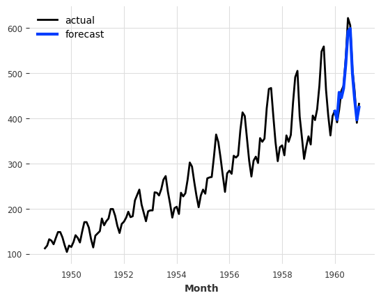
metadata: None# training a Exponential Smoothing model and plotting prediction
model = ExponentialSmoothing()
model.fit(train)
prediction = model.predict(len(val))
series.plot(label='actual')
prediction.plot(label='forecast', lw=3)
plt.legend();
series<TimeSeries (Month: 144, component: 1, sample: 1)> Size: 1kB
array([[[112.]],

       [[118.]],

       [[132.]],

       [[129.]],

       [[121.]],

       [[135.]],

       [[148.]],

       [[148.]],

       [[136.]],

       [[119.]],

...

       [[419.]],

       [[461.]],

       [[472.]],

       [[535.]],

       [[622.]],

       [[606.]],

       [[508.]],

       [[461.]],

       [[390.]],

       [[432.]]])
Coordinates:
* Month (Month) datetime64[ns] 1kB 1949-01-01 1949-02-01 ... 1960-12-01
* component (component) object 8B 'Passengers'
Dimensions without coordinates: sample
Attributes:
static_covariates: None
hierarchy: None
metadata: None# get order of first differencing: the higher of KPSS and ADF test results
result = adfuller(series.to_dataframe())
print('ADF Statistic: %f' % result[0])
print('p-value: %f' % result[1])
print('Critical Values:')
for key, value in result[4].items():
print('\t%s: %.3f' % (key, value))
if result[1] <= 0.05:
print("Reject the null hypothesis: The series is stationary")
else:
print("Fail to reject the null hypothesis: The series is non-stationary")ADF Statistic: 0.815369
p-value: 0.991880
Critical Values:
1%: -3.482
5%: -2.884
10%: -2.579
Fail to reject the null hypothesis: The series is non-stationary# exponential smoothing
m_expon = ExponentialSmoothing()
# prepare Prophet forecaster: multiplicative seas
m_prophet_m = Prophet(seasonality_mode="multiplicative")
# prepare Prophet forecaster: additive seas
m_prophet_a = Prophet(seasonality_mode="additive")
# prepare autoARIMA from StatsForecast
m_autoarima_stats = AutoARIMA(season_length=12)# list of models to be evaluated
models = [
m_expon,
m_prophet_m,
m_prophet_a,
m_autoarima_stats]## fit the chosen forecaster model and compute predictions
def eval_model(model, train, val):
t_start = time.perf_counter()
print("beginning: " + str(model))
# fit the model and compute predictions
res = model.fit(train)
forecast = model.predict(len(val))
# compute accuracy metrics and processing time
res_mape = mape(val, forecast)
res_mae = mae(val, forecast)
res_r2 = r2_score(val, forecast)
res_rmse = rmse(val, forecast)
res_rmsle = rmsle(val, forecast)
res_time = time.perf_counter() - t_start
res_accuracy = {"MAPE":res_mape, "MAE":res_mae, "R squared":-res_r2, "RMSE":res_rmse, "RMSLE":res_rmsle, "time":res_time}
results = [forecast, res_accuracy, res]
print("completed: " + str(model) + ":" + str(res_time) + "sec")
return resultseval_model(m_prophet_m, train, val)[1]beginning: Prophet(seasonality_mode=multiplicative)completed: Prophet(seasonality_mode=multiplicative):0.27867658200011647sec{'MAPE': np.float64(4.443829749162533),
'MAE': np.float64(21.908813279003937),
'R squared': np.float64(-0.8794305116779759),
'RMSE': np.float64(25.84359362409569),
'RMSLE': np.float64(0.05137792905621055),
'time': 0.27867658200011647}eval_model(m_autoarima_stats, train, val)[1]beginning: AutoARIMA(season_length=12)
completed: AutoARIMA(season_length=12):0.7895365719998608sec{'MAPE': np.float64(4.1796926177437514),
'MAE': np.float64(18.515823497791207),
'R squared': np.float64(-0.8967154852992124),
'RMSE': np.float64(23.919483693648484),
'RMSLE': np.float64(0.05350335125515268),
'time': 0.7895365719998608}Running all the models
# call the forecasters one after the other
model_predictions = [eval_model(model, train, val) for model in models]
beginning: ExponentialSmoothing()
completed: ExponentialSmoothing():0.12557467699980407sec
beginning: Prophet(seasonality_mode=multiplicative)completed: Prophet(seasonality_mode=multiplicative):0.13173181999991357sec
beginning: Prophet(seasonality_mode=additive)
completed: Prophet(seasonality_mode=additive):0.09849881199988886sec
beginning: AutoARIMA(season_length=12)
completed: AutoARIMA(season_length=12):0.37064578100012113sec# RUN the forecasters and tabulate their prediction accuracy and processing time
df_acc = pd.DataFrame.from_dict(model_predictions[0][1], orient="index")
df_acc.columns = [str(models[0])]
for i, m in enumerate(models):
if i > 0:
df = pd.DataFrame.from_dict(model_predictions[i][1], orient="index")
df.columns = [str(m)]
df_acc = pd.concat([df_acc, df], axis=1)
i +=1
pd.set_option("display.precision",3)
df_acc.style.highlight_min(color="lightgreen", axis=1).highlight_max(color="yellow", axis=1)| ExponentialSmoothing() | Prophet(seasonality_mode=multiplicative) | Prophet(seasonality_mode=additive) | AutoARIMA(season_length=12) | |
|---|---|---|---|---|
| MAPE | 2.803136 | 4.443830 | 6.614227 | 4.179693 |
| MAE | 13.382162 | 21.908813 | 33.434485 | 18.515823 |
| R squared | -0.947945 | -0.879431 | -0.665160 | -0.896715 |
| RMSE | 16.981068 | 25.843594 | 43.067799 | 23.919484 |
| RMSLE | 0.035501 | 0.051378 | 0.081915 | 0.053503 |
| time | 0.125575 | 0.131732 | 0.098499 | 0.370646 |
import logging

logging.getLogger("prophet").setLevel(logging.WARNING)
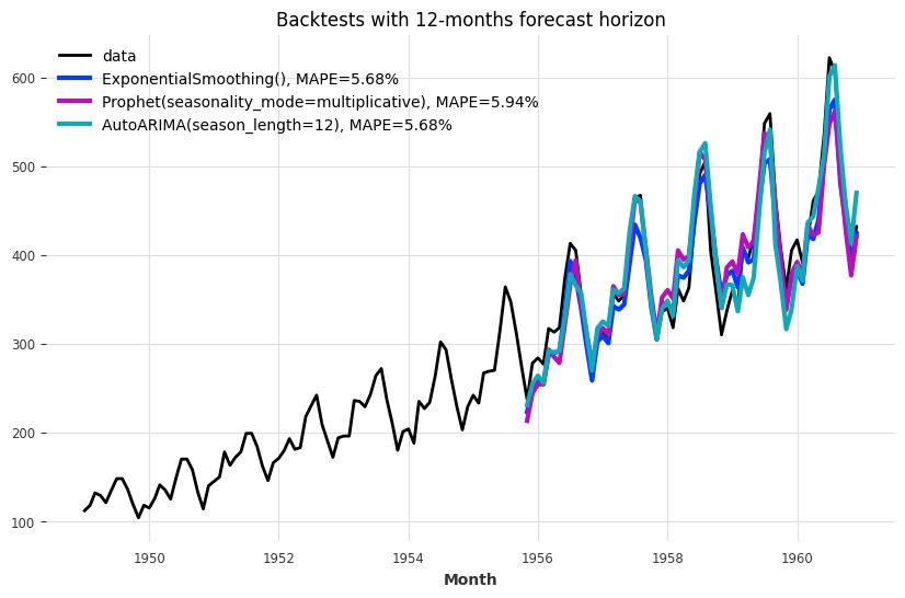
logging.getLogger("cmdstanpy").disabled=Truemodels_backtest = [m_expon, m_prophet_m, m_autoarima_stats]
backtests = [model.historical_forecasts(series, start=.5, forecast_horizon=12) for model in models_backtest]
plt.figure(figsize=(10, 6))
series.plot(label='data')
for i, m in enumerate(models_backtest):
err = mape(backtests[i], series)
backtests[i].plot(lw=3, label='{}, MAPE={:.2f}%'.format(m, err))
plt.title('Backtests with 12-months forecast horizon')
plt.legend()