# selection of orders of VAR: optimizing using information criteriamodel.select_order(15)results = model.fit(maxlags=15, ic='aic')lag_order = results.k_arprint("chosen VAR order is = "+str(lag_order))
chosen VAR order is = 3
Código
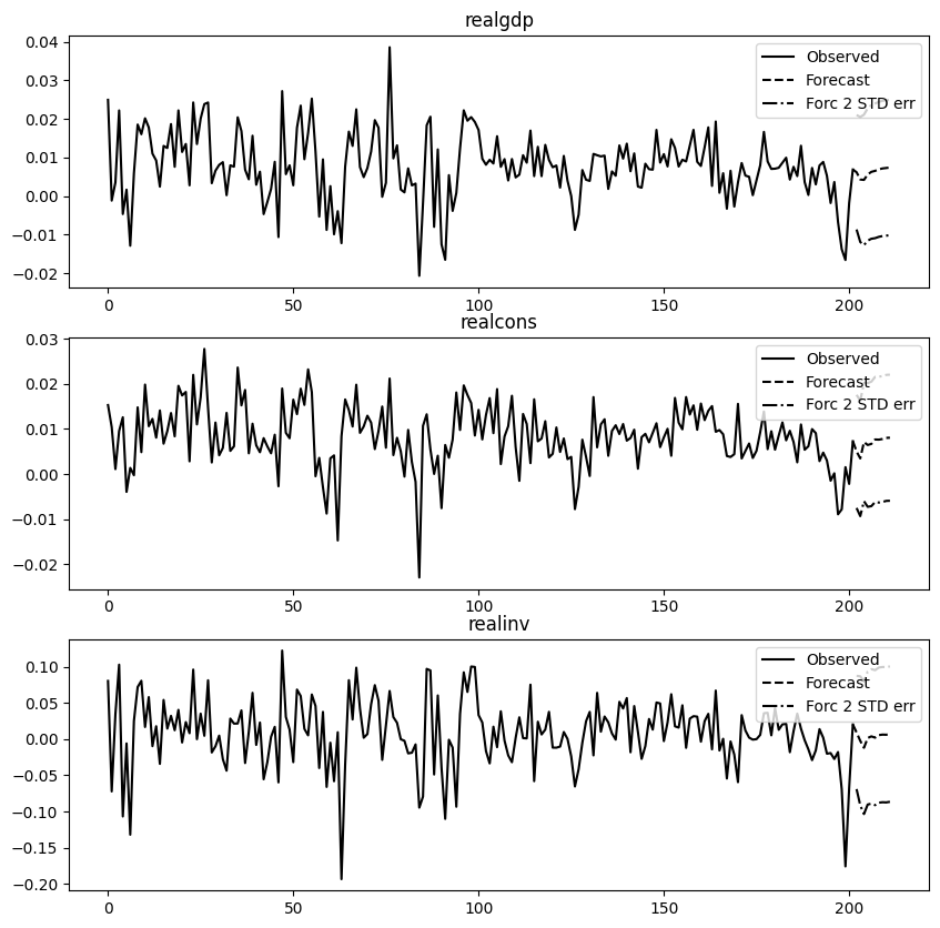
# forecasting: have to pass initial valuesresults.forecast(data.values[-lag_order:], 10)
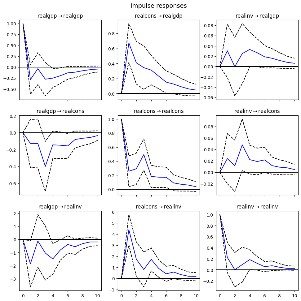
Impulse response function: how a system responds to a sudden change or impulse in its input in the time domain. In economics, and especially in contemporary macroeconomic modeling, impulse response functions are used to describe how the economy reacts over time to exogenous impulses, which economists usually call shocks, and are often modeled in the context of a vector autoregression.
Based on: - https://github.com/KidQuant/Pairs-Trading-With-Python/blob/master/PairsTrading.ipynb - https://www.programcreek.com/python/example/122726/statsmodels.tsa.stattools.coint - https://www.statsmodels.org/dev/generated/statsmodels.tsa.stattools.coint.html# - https://quantopian-archive.netlify.app/notebooks/notebooks/quantopian_notebook_145.html
Código
import pandas as pdimport numpy as npfrom statsmodels.tsa.stattools import cointfrom pandas_datareader import data as pdrimport datetimeimport yfinance as yfimport matplotlib.pyplot as plt
A note on how to detect cointegration
Steps:
Test for a unit root in each component series individually, using the univariate unit root tests, say ADF, KPSS, PP test.
In the case we don’t reject the null hypothesis of unit root, we can apply Engle-Granger test:
It works in two steps: first, a regression is estimated between the variables and the residuals are extracted. Second, a unit root test, such as the Augmented Dickey-Fuller (ADF) test, is applied to the residuals to check if they are stationary. If the residuals are stationary, the original variables are considered cointegrated.”
The coint function from statsmodels.tsa.stattools performs the Engle-Granger two-step cointegration test.
Simulating some example data
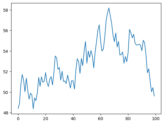
Simulating prices using cumulative returns;
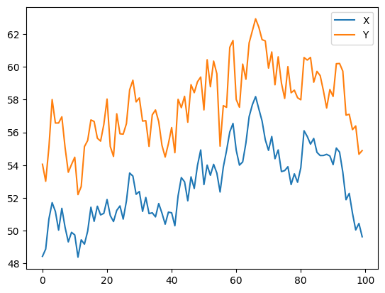
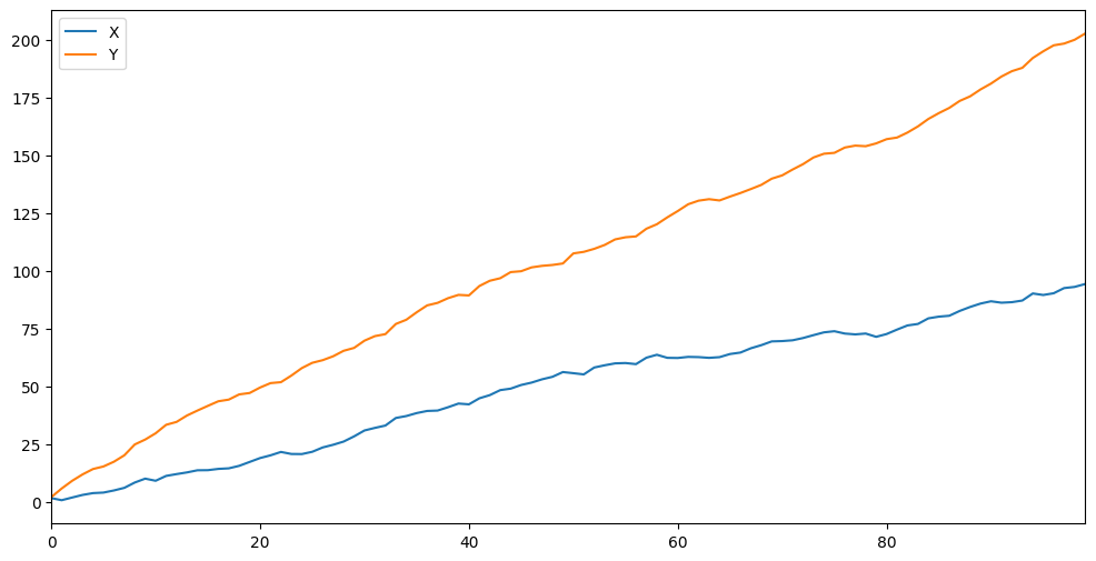
Now we generate Y. Remember that Y is supposed to have a deep economic link to X, so the price of Y should vary pretty similarly. We model this by taking X, shifting it up and adding some random noise drawn from a normal distribution.
Código
X_returns = np.random.normal(0, 1, 100) # generating random normal varX = pd.Series(np.cumsum(X_returns), name='X') +50X.plot()
Testing for cointegration. But first, we can compare cointegration vs correlation.
Código
X.corr(Y)
np.float64(0.9273678099454663)
Código
# compute the p-value of the cointegration test# Test for no-cointegration of a univariate equation as H0# will inform us as to whether the spread btwn the 2 timeseries is stationary# around its meanscore, pvalue, _ = coint(X,Y)print(pvalue)
1.5239505499170159e-09
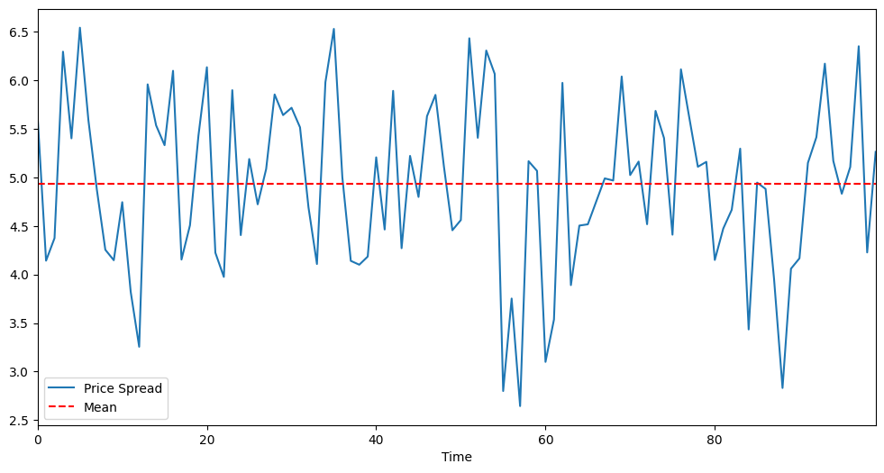
With a low value for test p-value, we cannot reject the cointegration the hypothesis of residuals being I(0) - stationarity.
Código
plt.figure(figsize=(12,6))(Y - X).plot() # Plot the spreadplt.axhline((Y - X).mean(), color='red', linestyle='--') # Add the meanplt.xlabel('Time')plt.xlim(0,99)plt.legend(['Price Spread', 'Mean']);
# function to build log returns from a dataframedef log_returns(df):import numpy as np df_ = df.copy()for stock in df.columns: df_[stock] = np.log(df_[stock]).diff()return df_.dropna()
Código
# applying the functiondaily_returns = log_returns(df)daily_returns
Ticker
AAPL
ADBE
AMD
EBAY
HPQ
IBM
MSFT
ORCL
QCOM
SPY
Date
2013-01-03
-0.012703
-0.015508
-0.015937
-0.021502
0.007958
-0.005515
-0.013487
-0.011014
-0.004644
-0.002262
2013-01-04
-0.028250
0.010016
0.039375
0.006272
0.000000
-0.006577
-0.018893
0.008706
-0.014850
0.004382
2013-01-07
-0.005900
-0.004995
0.030421
0.013736
0.001980
-0.004391
-0.001872
-0.005214
0.007999
-0.002736
2013-01-08
0.002688
0.005258
0.000000
-0.015633
0.014398
-0.001399
-0.005259
0.000290
-0.001563
-0.002881
2013-01-09
-0.015752
0.013542
-0.015095
0.001517
0.029452
-0.002856
0.005634
0.000581
0.015063
0.002539
...
...
...
...
...
...
...
...
...
...
...
2017-12-22
0.000000
0.002517
-0.032667
-0.001323
0.000470
0.006579
0.000117
0.001691
0.005267
-0.000262
2017-12-26
-0.025697
-0.003205
-0.007619
0.004755
-0.001412
0.002162
-0.001287
0.001477
-0.006665
-0.001197
2017-12-27
0.000176
0.005260
0.006670
-0.008736
0.001882
0.001961
0.003623
-0.001055
0.003726
0.000486
2017-12-28
0.002810
0.001083
0.001898
0.008208
-0.005658
0.005925
0.000117
0.002951
-0.002482
0.002055
2017-12-29
-0.010873
-0.001767
-0.025926
-0.004758
-0.006641
-0.004033
-0.002102
-0.005063
-0.005607
-0.003778
1258 rows × 10 columns
Código
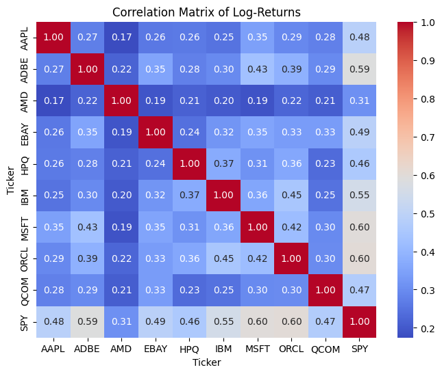
# matrix correlation of log-returnsimport seaborn as snscorrelation_matrix = daily_returns.corr()plt.figure(figsize=(8, 6))sns.heatmap(correlation_matrix, annot=True, cmap='coolwarm', fmt=".2f")plt.title('Correlation Matrix of Log-Returns')plt.show()
Explanation of the meaning of “trading the spread”:
In a cointegrated pair trading strategy, ‘trading the spread’ refers to exploiting the long-term, statistically stable relationship between the prices of two cointegrated assets. Here’s a breakdown:
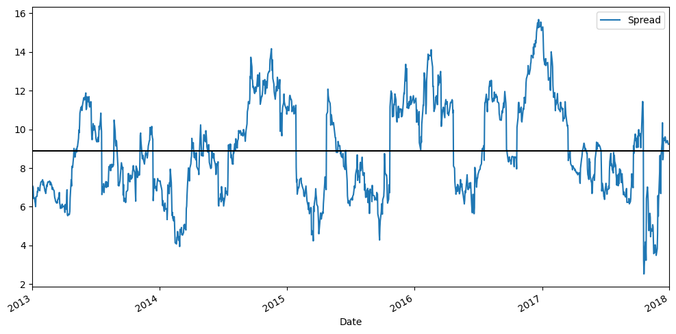
Cointegrated Pair: When two (or more) non-stationary time series are cointegrated, it means they move together in the long run, and a linear combination of them is stationary. This stationary linear combination is often referred to as the ‘spread’ or ‘error correction term’. Even though individual asset prices might wander, their relationship tends to revert to a mean.
The Spread: The ‘spread’ is typically defined as the difference between the price of one asset and a scaled price of the other asset (e.g., Spread = Price_Y - beta * Price_X, where beta is the hedge ratio obtained from a regression, as we saw with b for ADBE and MSFT). Because the assets are cointegrated, this spread is expected to be stationary, meaning it will fluctuate around a constant mean.
Trading the Spread Strategy (Mean Reversion):
Execution:
When the spread deviates significantly above its historical mean (meaning one asset is relatively overvalued compared to the other), you would sell the overvalued asset and buy the undervalued asset. For example, if Price_Y - beta * Price_X is high, you’d sell Y and buy X.
Closing Position: The goal is to profit when the spread reverts to its mean. Once the spread returns to its average, you would close both positions, realizing a profit.