We will start by picking up some data from Yahoo Finance APIs
Código
import yfinance as yf#getting historic stock data from yfinancestocks_list = ['BBDC4.SA', 'ITUB4.SA','SANB4.SA', 'BBAS3.SA']data = yf.download(stocks_list, period='5y')['Close']data
Ticker
BBAS3.SA
BBDC4.SA
ITUB4.SA
SANB4.SA
Date
2020-11-23
11.589112
14.348302
20.156155
14.215531
2020-11-24
11.897979
14.993038
20.721098
14.784431
2020-11-25
11.864407
14.799619
20.476992
15.099722
2020-11-26
11.676399
14.559301
20.044575
15.264223
2020-11-27
11.619331
14.442083
20.198011
15.181969
...
...
...
...
...
2025-11-14
22.440001
19.469999
40.599998
17.500000
2025-11-17
22.500000
19.320000
40.299999
17.270000
2025-11-18
21.879999
19.090000
40.099998
17.330000
2025-11-19
21.580000
18.900000
39.849998
17.129999
2025-11-21
22.000000
18.790001
39.970001
17.150000
1247 rows × 4 columns
Then we transform data to build log returns:
Código
# function to build log returns from a dataframedef log_returns(df):import numpy as np df_ = df.copy()for stock in df.columns: df_[stock] = np.log(df_[stock]).diff()return df_.dropna()
Código
# applying the functiondaily_returns = log_returns(data)daily_returns
Ticker
BBAS3.SA
BBDC4.SA
ITUB4.SA
SANB4.SA
Date
2020-11-24
0.026302
0.043954
0.027643
0.039240
2020-11-25
-0.002826
-0.012985
-0.011851
0.021102
2020-11-26
-0.015973
-0.016371
-0.021343
0.010835
2020-11-27
-0.004899
-0.008084
0.007626
-0.005403
2020-11-30
-0.021908
-0.013895
-0.013909
-0.050462
...
...
...
...
...
2025-11-14
-0.002670
-0.000513
0.003949
0.014969
2025-11-17
0.002670
-0.007734
-0.007417
-0.013230
2025-11-18
-0.027942
-0.011976
-0.004975
0.003468
2025-11-19
-0.013806
-0.010003
-0.006254
-0.011608
2025-11-21
0.019275
-0.005837
0.003007
0.001167
1246 rows × 4 columns
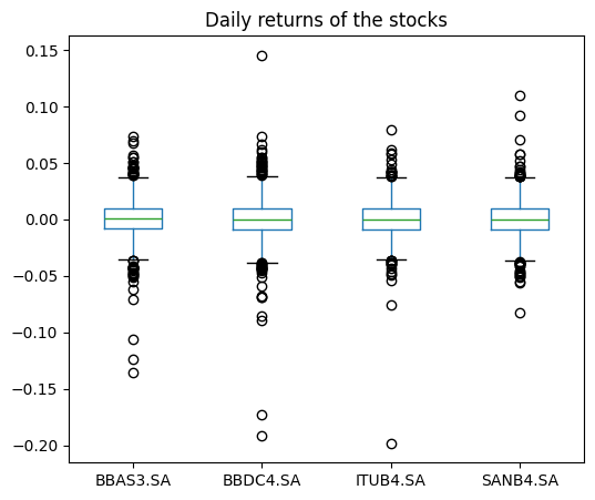
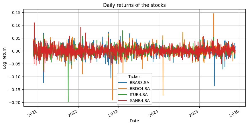
Then we can plot log returns and understand about conditional hererocedasticy and distribution
Código
import matplotlib.pyplot as plt# Boxplot of daily returnsdaily_returns.boxplot(figsize=(6, 5), grid=False)plt.title("Daily returns of the stocks");
Código
# Lineplot of daily returnsdaily_returns.plot(figsize=(10, 5))plt.title("Daily returns of the stocks")plt.xlabel("Date")plt.ylabel("Log Return")plt.grid(True)plt.show();
Código
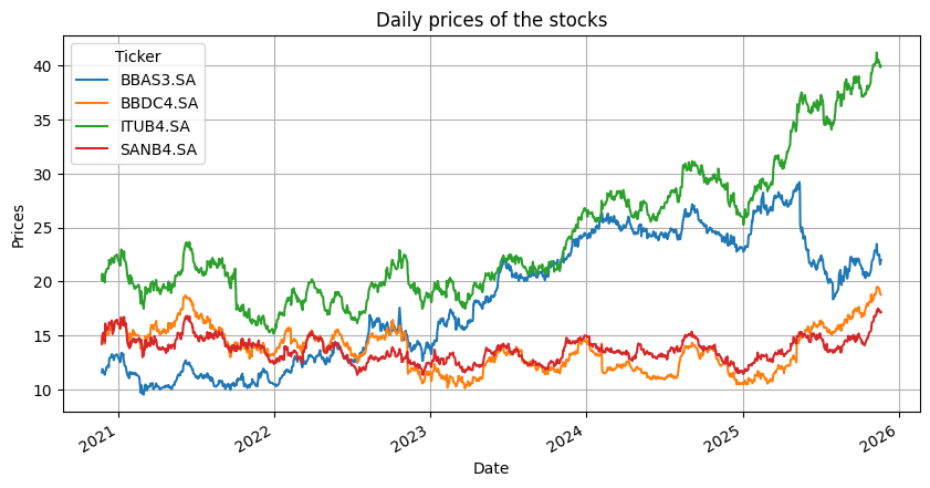
# Lineplot of pricesdata.plot(figsize=(10, 5))plt.title("Daily prices of the stocks")plt.xlabel("Date")plt.ylabel("Prices")plt.grid(True)plt.show();
Código
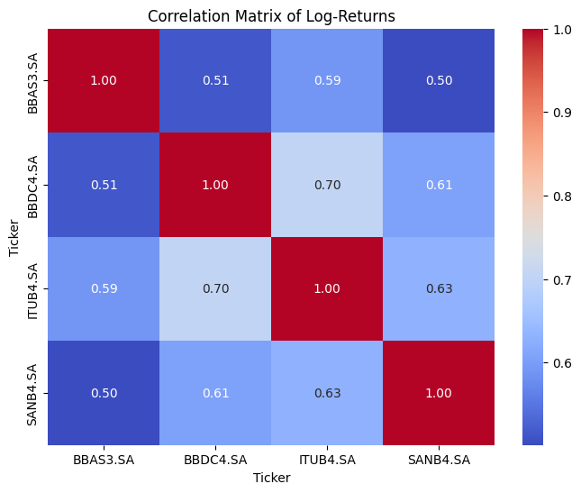
# matrix correlation of log-returnsimport seaborn as snscorrelation_matrix = daily_returns.corr()plt.figure(figsize=(8, 6))sns.heatmap(correlation_matrix, annot=True, cmap='coolwarm', fmt=".2f")plt.title('Correlation Matrix of Log-Returns')plt.show()
Código
# calculate historical volatility of log_returns (generated by AI)def historical_volatility(log_returns, annualizing_factor=252):"""Calculates the historical volatility of log returns. Args: log_returns: A pandas DataFrame of daily log returns. annualizing_factor: The number of trading days in a year (default is 252). Returns: A pandas Series of annualized historical volatility for each asset. """import numpy as npimport pandas as pd daily_volatility = log_returns.std() annualized_volatility = daily_volatility * np.sqrt(annualizing_factor)return annualized_volatility# Calculate historical volatility for the daily returnshistorical_vol = historical_volatility(daily_returns)print("\nHistorical Volatility:")historical_vol
Historical Volatility:
0
Ticker
BBAS3.SA
0.275599
BBDC4.SA
0.303753
ITUB4.SA
0.257582
SANB4.SA
0.269779
Now let’s calculate CAPM model for the assets. For this we need to pick up the market return
Código
#getting historic stock data from yfinancestocks_list = ['^BVSP']ibov = yf.download(stocks_list, period='5y')['Close']mkt_returns = log_returns(ibov)mkt_returns = mkt_returns.rename(columns={'^BVSP': 'mkt_return'})
Código
mkt_returns
Ticker
mkt_return
Date
2020-11-24
0.022168
2020-11-25
0.003156
2020-11-26
0.000853
2020-11-27
0.003152
2020-11-30
-0.015374
...
...
2025-11-14
0.003665
2025-11-17
-0.004741
2025-11-18
-0.003005
2025-11-19
-0.007316
2025-11-21
-0.003940
1246 rows × 1 columns
Código
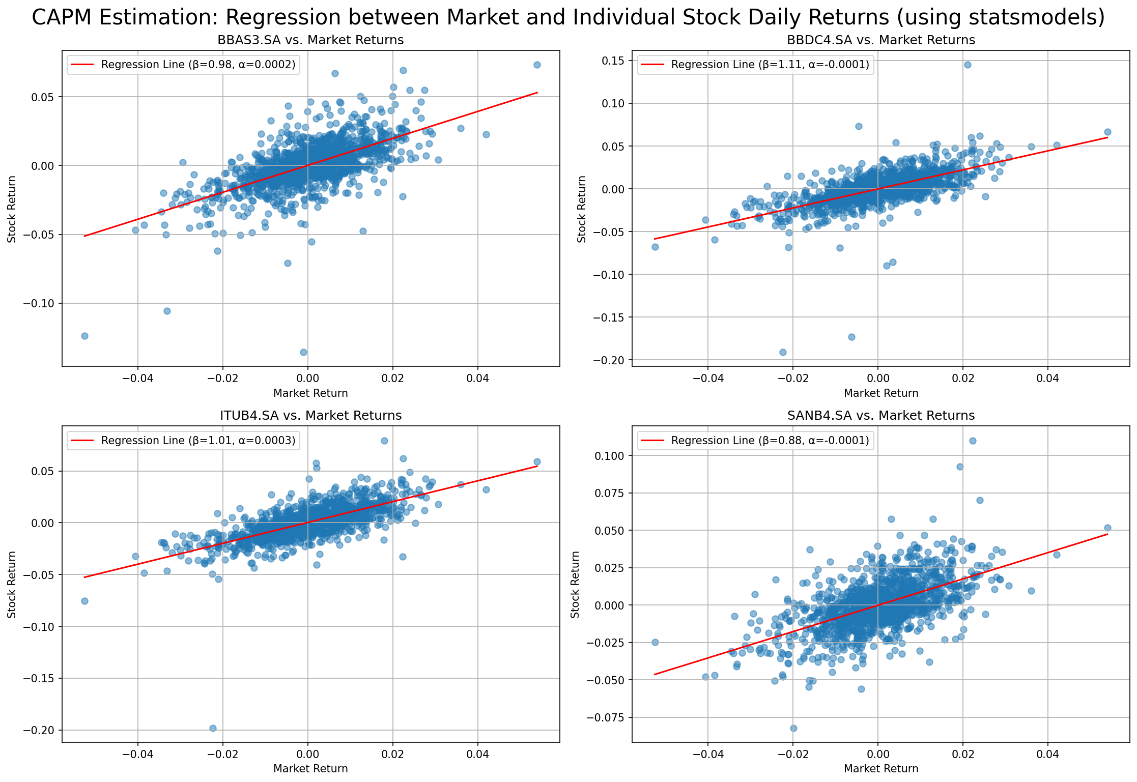
# prompt: capm model between log_returns and mkt_returnsimport statsmodels.api as smimport pandas as pdimport numpy as npimport matplotlib.pyplot as pltbeta_sm, alpha_sm =dict(), dict()# Loop through each stock to perform regressionfor stock in daily_returns.columns:# Define dependent and independent variables y = daily_returns[stock] X = mkt_returns['mkt_return']# Add a constant for the intercept (alpha) X = sm.add_constant(X)# Perform the regression model = sm.OLS(y, X).fit()# Extract beta and alpha beta_sm[stock] = model.params['mkt_return'] alpha_sm[stock] = model.params['const']# Print the regression results summaryprint(f"\nCAPM Regression Results for {stock}:")print(model.summary())print("\nBetas from statsmodels:")print(beta_sm)print("\nAlphas from statsmodels:")print(alpha_sm)
# Plotting the regressions using statsmodelsfig, axes = plt.subplots(2, 2, dpi=150, figsize=(15, 10))axes = axes.flatten()for stock in daily_returns.columns: idx = daily_returns.columns.get_loc(stock)if stock in beta_sm and stock in alpha_sm: X = mkt_returns['mkt_return'] y = daily_returns[stock]# Scatter plot axes[idx].scatter(X, y, alpha=0.5)# Add the regression line using the statsmodels results# Create a range of market return values for the line mkt_return_range = np.linspace(X.min(), X.max(), 100) regression_line = alpha_sm[stock] + beta_sm[stock] * mkt_return_range axes[idx].plot(mkt_return_range, regression_line, color='red', label=f'Regression Line (β={beta_sm[stock]:.2f}, α={alpha_sm[stock]:.4f})') axes[idx].set_title(f'{stock} vs. Market Returns') axes[idx].set_xlabel('Market Return') axes[idx].set_ylabel('Stock Return') axes[idx].legend() axes[idx].grid(True)else: axes[idx].set_title(f'{stock} vs. Market Returns - Data Missing') axes[idx].text(0.5, 0.5, 'Data Missing', horizontalalignment='center', verticalalignment='center', transform=axes[idx].transAxes)plt.tight_layout()plt.suptitle("CAPM Estimation: Regression between Market and Individual Stock Daily Returns (using statsmodels)", size=20, y=1.02)plt.show()
Código
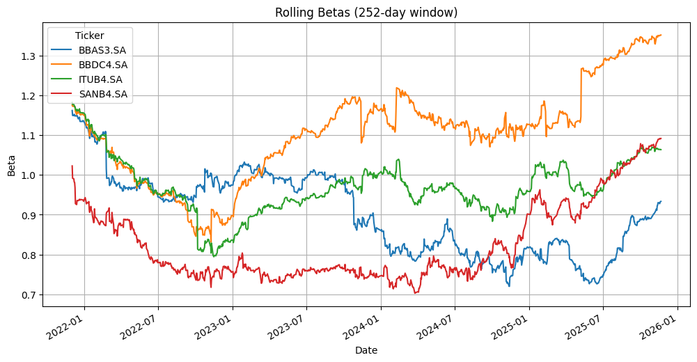
# prompt: rolling betas camp for daily_returns using statsmodels regressiondef rolling_betas_camp(daily_returns, mkt_returns, window):""" Calculates rolling betas for a list of stocks against the market using statsmodels OLS. Args: daily_returns (pd.DataFrame): DataFrame of daily log returns for the stocks. mkt_returns (pd.DataFrame): DataFrame of daily log returns for the market. window (int): The size of the rolling window. Returns: pd.DataFrame: DataFrame containing the rolling betas for each stock. """ rolling_betas = pd.DataFrame(index=daily_returns.index, columns=daily_returns.columns)for stock in daily_returns.columns:for i inrange(window, len(daily_returns)):# Define the rolling window window_returns = daily_returns[stock].iloc[i-window:i] window_mkt_returns = mkt_returns['mkt_return'].iloc[i-window:i]# Ensure there are enough data points in the windowiflen(window_returns) == window andlen(window_mkt_returns) == window:# Define dependent and independent variables y = window_returns X = window_mkt_returns# Add a constant for the intercept (alpha) X = sm.add_constant(X)# Perform the regressiontry: model = sm.OLS(y, X).fit()# Store the beta value rolling_betas.loc[daily_returns.index[i], stock] = model.params['mkt_return']exceptExceptionas e:# Handle cases where regression might fail (e.g., no variation in data)print(f"Regression failed for {stock} at index {daily_returns.index[i]}: {e}") rolling_betas.loc[daily_returns.index[i], stock] = np.nanreturn rolling_betas# Calculate rolling betas with a window of 252 trading days (approx 1 year)rolling_betas = rolling_betas_camp(daily_returns, mkt_returns, window=252)print("\nRolling Betas:")print(rolling_betas.tail())# Plot the rolling betasrolling_betas.plot(figsize=(12, 6))plt.title('Rolling Betas (252-day window)')plt.xlabel('Date')plt.ylabel('Beta')plt.grid(True)plt.show()
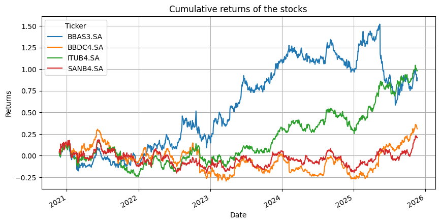
def calculate_cumulative_returns(returns):""" Calculates cumulative returns from a series of simple returns. Args: returns: A pandas Series or NumPy array of simple returns. Returns: A pandas Series or NumPy array of cumulative returns. """ cumulative_returns = (1+ daily_returns_level).cumprod() -1return cumulative_returns# Example usage:# Assuming you have a pandas Series of daily returns called 'daily_returns'# Example Datacumulative_returns = calculate_cumulative_returns(returns)print(cumulative_returns)
# Lineplot of daily returnscumulative_returns.plot(figsize=(10, 5))plt.title("Cumulative returns of the stocks")plt.xlabel("Date")plt.ylabel("Returns")plt.grid(True)plt.show();
Código
np.exp(mkt_returns)-1
Ticker
mkt_return
Date
2020-11-24
0.022416
2020-11-25
0.003161
2020-11-26
0.000854
2020-11-27
0.003157
2020-11-30
-0.015257
...
...
2025-11-14
0.003671
2025-11-17
-0.004729
2025-11-18
-0.003000
2025-11-19
-0.007290
2025-11-21
-0.003932
1246 rows × 1 columns
Código
mkt_returns
Ticker
mkt_return
Date
2020-11-24
0.022168
2020-11-25
0.003156
2020-11-26
0.000853
2020-11-27
0.003152
2020-11-30
-0.015374
...
...
2025-11-14
0.003665
2025-11-17
-0.004741
2025-11-18
-0.003005
2025-11-19
-0.007316
2025-11-21
-0.003940
1246 rows × 1 columns
Código
# Estimate the expected return of the market using the daily returnsER =dict()rf =0.1383#mkt_returns_level = np.exp(mkt_returns)-1rm = mkt_returns.mean()*252for k in daily_returns.columns:# Calculate return for every security using CAPM ER[k] = rf + beta_sm[k] * (rm-rf)print("Expected return based on CAPM model for {} is {}%".format(k, round(ER[k]*100, 2)))# Calculating historic returnsprint('Return based on historical data for {} is {}%'.format(k, round(daily_returns[k].mean() *100*252, 2)))
Expected return based on CAPM model for BBAS3.SA is Ticker
mkt_return    7.52
dtype: float64%
Return based on historical data for BBAS3.SA is 12.96%
Expected return based on CAPM model for BBDC4.SA is Ticker
mkt_return    6.67
dtype: float64%
Return based on historical data for BBDC4.SA is 5.45%
Expected return based on CAPM model for ITUB4.SA is Ticker
mkt_return    7.36
dtype: float64%
Return based on historical data for ITUB4.SA is 13.85%
Expected return based on CAPM model for SANB4.SA is Ticker
mkt_return    8.17
dtype: float64%
Return based on historical data for SANB4.SA is 3.8%
Código
rm
np.float64(0.07393662034276567)
Código
# prompt: calculate sharpe ratio of daily_returnsdef sharpe_ratio(returns, risk_free_rate=0):""" Calculates the Sharpe Ratio for a given series of returns. Args: returns (pd.Series or np.array): A series or array of returns. risk_free_rate (float): The risk-free rate of return (default is 0). Should be on the same frequency as the returns. Returns: float: The Sharpe Ratio. """ excess_returns = returns - risk_free_ratereturn excess_returns.mean() / excess_returns.std()# Calculate Sharpe Ratio for each stocksharpe_ratios = {}annualized_risk_free_rate = rf # Using the already defined annualized risk-free rate# Assuming the risk-free rate is given as an annual rate, we need to convert it# to the same frequency as the daily returns. For daily returns, we take the# daily equivalent risk-free rate.# daily_risk_free_rate = (1 + annualized_risk_free_rate)**(1/252) - 1# A simpler approximation is annual_rate / 252 for small rates.# Let's use the approximation for simplicity here, assuming rf is an annualized rate.daily_risk_free_rate = annualized_risk_free_rate /252for stock in daily_returns.columns: sharpe_ratios[stock] = sharpe_ratio(daily_returns[stock], daily_risk_free_rate)print("\nSharpe Ratios:")for stock, ratio in sharpe_ratios.items():print(f"{stock}: {ratio:.4f}")
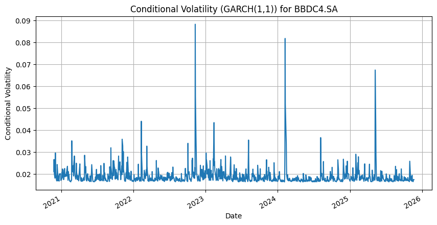
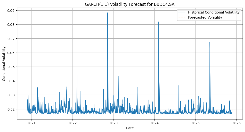
# prompt: Garch model volatility forecast for daily_returns!pip install archfrom arch import arch_model# Select one stock to model (e.g., BBDC4.SA)stock_to_model ='BBDC4.SA'returns_to_model = daily_returns[stock_to_model]# Fit a GARCH(1, 1) model# The `vol='GARCH'` specifies the GARCH process# The `p=1` and `q=1` specify the orders of the AR and MA terms for the variance equationam = arch_model(returns_to_model, vol='Garch', p=1, q=1)res = am.fit(update_freq=5)# Print the model summaryprint(res.summary())# Plot the conditional variance (volatility)fig = res.conditional_volatility.plot(figsize=(10, 5))plt.title(f'Conditional Volatility (GARCH(1,1)) for {stock_to_model}')plt.xlabel('Date')plt.ylabel('Conditional Volatility')plt.grid(True)plt.show()# Make a forecast of the conditional volatility# Forecast for the next 5 daysforecast_horizon =5forecasts = res.forecast(horizon=forecast_horizon)# The forecast object contains different types of forecasts.# We are interested in the volatility forecasts.# 'h.0' is the mean of the conditional variance forecast# 'h.1' are the quantiles (if calculated)# 'variance' is the forecast of the conditional variance itself# We need to take the square root of the variance forecast to get volatilityforecast_volatility = np.sqrt(forecasts.variance)# The forecast is given for the horizons starting from the last observation.# Get the index for the forecastlast_date = returns_to_model.index[-1]forecast_dates = pd.date_range(start=last_date, periods=forecast_horizon +1, freq='D')[1:] # +1 and [1:] to exclude the last historical dateprint(f'\nGARCH(1,1) Volatility Forecast for {stock_to_model} (next {forecast_horizon} days):')forecast_df = pd.DataFrame(forecast_volatility.iloc[-1].values, index=forecast_dates, columns=['Forecasted Volatility'])print(forecast_df)# Optional: Plot the historical conditional volatility and the forecastplt.figure(figsize=(12, 6))plt.plot(res.conditional_volatility.index, res.conditional_volatility, label='Historical Conditional Volatility')plt.plot(forecast_df.index, forecast_df['Forecasted Volatility'], label='Forecasted Volatility', linestyle='--')plt.title(f'GARCH(1,1) Volatility Forecast for {stock_to_model}')plt.xlabel('Date')plt.ylabel('Conditional Volatility')plt.legend()plt.grid(True)plt.show()
Requirement already satisfied: arch in /usr/local/lib/python3.12/dist-packages (8.0.0)
Requirement already satisfied: numpy<3,>=1.22.3 in /usr/local/lib/python3.12/dist-packages (from arch) (2.0.2)
Requirement already satisfied: pandas>=1.4.0 in /usr/local/lib/python3.12/dist-packages (from arch) (2.2.2)
Requirement already satisfied: scipy>=1.8 in /usr/local/lib/python3.12/dist-packages (from arch) (1.16.3)
Requirement already satisfied: statsmodels>=0.13.0 in /usr/local/lib/python3.12/dist-packages (from arch) (0.14.5)
Requirement already satisfied: packaging in /usr/local/lib/python3.12/dist-packages (from arch) (25.0)
Requirement already satisfied: python-dateutil>=2.8.2 in /usr/local/lib/python3.12/dist-packages (from pandas>=1.4.0->arch) (2.9.0.post0)
Requirement already satisfied: pytz>=2020.1 in /usr/local/lib/python3.12/dist-packages (from pandas>=1.4.0->arch) (2025.2)
Requirement already satisfied: tzdata>=2022.7 in /usr/local/lib/python3.12/dist-packages (from pandas>=1.4.0->arch) (2025.2)
Requirement already satisfied: patsy>=0.5.6 in /usr/local/lib/python3.12/dist-packages (from statsmodels>=0.13.0->arch) (1.0.2)
Requirement already satisfied: six>=1.5 in /usr/local/lib/python3.12/dist-packages (from python-dateutil>=2.8.2->pandas>=1.4.0->arch) (1.17.0)
Iteration:      5,   Func. Count:     39,   Neg. LLF: -3154.1819099755176
Iteration:     10,   Func. Count:     67,   Neg. LLF: -3188.1621902352554
Optimization terminated successfully    (Exit mode 0)
            Current function value: -3188.16219023508
            Iterations: 10
            Function evaluations: 67
            Gradient evaluations: 10
                     Constant Mean - GARCH Model Results
==============================================================================
Dep. Variable:               BBDC4.SA   R-squared:                       0.000
Mean Model:             Constant Mean   Adj. R-squared:                  0.000
Vol Model:                      GARCH   Log-Likelihood:                3188.16
Distribution:                  Normal   AIC:                          -6368.32
Method:            Maximum Likelihood   BIC:                          -6347.81
                                        No. Observations:                 1246
Date:                Mon, Nov 24 2025   Df Residuals:                     1245
Time:                        00:53:16   Df Model:                            1
                                  Mean Model
=============================================================================
                 coef    std err          t      P>|t|       95.0% Conf. Int.
-----------------------------------------------------------------------------
mu         7.8979e-04  7.154e-04      1.104      0.270 [-6.125e-04,2.192e-03]
                              Volatility Model
============================================================================
                 coef    std err          t      P>|t|      95.0% Conf. Int.
----------------------------------------------------------------------------
omega      1.7393e-04  5.969e-05      2.914  3.571e-03 [5.694e-05,2.909e-04]
alpha[1]       0.2035      0.125      1.627      0.104  [-4.170e-02,  0.449]
beta[1]        0.3491      0.175      1.994  4.618e-02   [5.922e-03,  0.692]
============================================================================

Covariance estimator: robust
# prompt: value at risk for daily_returns using volatility modelsdef calculate_value_at_risk(returns, confidence_level=0.95, model='historical', volatility_model=None):""" Calculates Value at Risk (VaR) for a series of returns. Args: returns (pd.Series): A series of returns. confidence_level (float): The confidence level for the VaR (e.g., 0.95 for 95%). model (str): The VaR model to use. Options: 'historical', 'parametric' (uses normal distribution), 'parametric_garch'. volatility_model: Fitted volatility model object (e.g., from `arch_model.fit()`) if model is 'parametric_garch'. Returns: float: The calculated VaR. """ alpha =1- confidence_levelif model =='historical':# Historical VaR: VaR is the quantile of historical returns VaR =-np.percentile(returns, alpha *100)elif model =='parametric':# Parametric VaR (Normal Distribution): VaR = - (mean + Z * std_dev)# Assuming mean is close to zero for daily returns, VaR approx -Z * std_dev# Z is the z-score corresponding to the confidence levelfrom scipy.stats import norm mean_return = returns.mean() std_dev_return = returns.std() z_score = norm.ppf(alpha) VaR =-(mean_return + z_score * std_dev_return)elif model =='parametric_garch'and volatility_model isnotNone:# Parametric VaR (using GARCH forecasted volatility)from scipy.stats import norm# Get the last conditional volatility from the GARCH model# This assumes you are calculating VaR for the next period based on the model forecasted_volatility = volatility_model.conditional_volatility.iloc[-1] mean_return = returns.mean() # You could potentially use forecasted mean if your model predicts it z_score = norm.ppf(alpha) VaR =-(mean_return + z_score * forecasted_volatility)else:raiseValueError("Invalid VaR model specified or missing volatility_model for 'parametric_garch'.")return VaR# --- Calculate VaR using different models ---# Select the stock for VaR calculationstock_for_var ='BBDC4.SA'returns_for_var = daily_returns[stock_for_var]# 1. Historical VaR (e.g., 95% confidence)var_historical_95 = calculate_value_at_risk(returns_for_var, confidence_level=0.95, model='historical')print(f"\nHistorical VaR (95%) for {stock_for_var}: {var_historical_95:.4f}")var_historical_99 = calculate_value_at_risk(returns_for_var, confidence_level=0.99, model='historical')print(f"Historical VaR (99%) for {stock_for_var}: {var_historical_99:.4f}")# 2. Parametric VaR (Normal Distribution)var_parametric_95 = calculate_value_at_risk(returns_for_var, confidence_level=0.95, model='parametric')print(f"\nParametric VaR (Normal, 95%) for {stock_for_var}: {var_parametric_95:.4f}")var_parametric_99 = calculate_value_at_risk(returns_for_var, confidence_level=0.99, model='parametric')print(f"Parametric VaR (Normal, 99%) for {stock_for_var}: {var_parametric_99:.4f}")# 3. Parametric VaR (using GARCH(1,1) volatility)# We need the fitted GARCH model object ('res' from the previous cell)if'res'inglobals(): # Check if the 'res' object exists var_parametric_garch_95 = calculate_value_at_risk(returns_for_var, confidence_level=0.95, model='parametric_garch', volatility_model=res)print(f"\nParametric VaR (GARCH(1,1) Volatility, 95%) for {stock_for_var}: {var_parametric_garch_95:.4f}") var_parametric_garch_99 = calculate_value_at_risk(returns_for_var, confidence_level=0.99, model='parametric_garch', volatility_model=res)print(f"Parametric VaR (GARCH(1,1) Volatility, 99%) for {stock_for_var}: {var_parametric_garch_99:.4f}")else:print("\nSkipping GARCH-based VaR calculation as the GARCH model ('res') is not fitted in this session.")
Historical VaR (95%) for BBDC4.SA: 0.0273
Historical VaR (99%) for BBDC4.SA: 0.0437

Parametric VaR (Normal, 95%) for BBDC4.SA: 0.0313
Parametric VaR (Normal, 99%) for BBDC4.SA: 0.0443

Parametric VaR (GARCH(1,1) Volatility, 95%) for BBDC4.SA: 0.0285
Parametric VaR (GARCH(1,1) Volatility, 99%) for BBDC4.SA: 0.0404